Modeling Caffeine Metabolism - time offset

What’s the next level of complexity to add to our model? As noted previously, our model is not able to generate an arbitrary caffeine schedule. Let’s add functionality to enable it to do so!

What do we need in order to do this? What we would like to do is to be able to simulate a single day as a combination of caffeine inputs at arbitrary times during the day. We would then like to repeat the day periodically. To accomplish this, we need the ability to add a time offset to a dose delivered every 24 hours. This enables us to construct a day out of a combination of different doses with different time offsets, i.e. a 100 mg dose at 9 am and then a 50 mg dose at 4 pm.

Let’s first derive an expression for a periodic dose of $d$ milligrams delivered every $a$ hours with a time offset (delay) from $t=0$ of $t_0$. As done previously, we can construct an expression for $f(t)$, the metabolically active amount at time $t$. We note that before $t_0$, the caffeine content will be zero as no dosing has started.

For $t \ge t_0$, this case is similar to the problem we have already solved but shifted in time by $t_0$. We can write out our sum of exponential terms (noting the time offset):

where $n$ corresponds to the last consumption event before time $t$. We can figure out what $n$ is by looking at the timing of events. There are no events before $t_0$. Afterwards, events occur every $a$ hours. To account for the dead time caused by the offset, we simply subtract it from the total time and figure out how many events happened every $a$ hours after that. Thus, we find that $n=\left\lfloor {\frac{t-t_0}{a}}\right\rfloor$.

We note that this expression is identical to our previous expression but with $t$ replaced by $t-t_0$. Thus, the final sum will be:

Thus, we have our overall expression for $f(t)$:

We have a simple expression for a repeated dose with a given offset. Now, we’d like the ability to build an arbitrary day out of such doses. So, let us consider doses $1, 2, \ldots, m$ with dose size $d_1, d_2, \ldots, d_m$, offset $t_1, t_2, \ldots, t_m$ and periodicity $a_1, a_2, \ldots, a_m$.

We can sum together these individual terms to construct the general expression. For $j=1,2,\ldots, m$:

Note that the $n_j$ values must be recalculated for every $j$.

To summarize so far, what we’ve done is constructed a sum of multiple different dosing schedules to be able to construct an arbitrary caffeine dosing schedule. We can implement these results in MATLAB as before. Note that we add a special case in the code for when $a=0$. This situation is nonphysical as it is equivalent to infinite consumption. We use $a=0$ (durationBetween in the code) as a magic number to indicate a non-repeating dosage. We will return to this later. First, the code:

function [ content ] = caffeineOffset( time, caffeineContent, durationBetween, offset )
    halfLife = 5.7;
    tau = halfLife/log(2);
    n = floor((time-offset)/durationBetween);

    if time < offset
        content = 0;
    elseif durationBetween == 0
        content = caffeineContent * exp(-(time-offset)/tau);
    else
        content = caffeineContent * exp(-(time-offset)/tau) * ((1-exp(durationBetween * (n+1)/tau))/(1-exp(durationBetween/tau)));    
    end
end

function [ content ] = caffeineOffsetList( time, caffeineContent, durationBetween, offset )
    %time is list of times
    %caffeineContent, durationBetween, and offset are lists of the same length    
    content = zeros(1,length(time));
    for i = 1:length(time)
        content(i) = 0;
        for j = 1:length(caffeineContent)
            content(i) = content(i) + caffeineOffset(time(i),caffeineContent(j),durationBetween(j),offset(j));
        end                
    end    
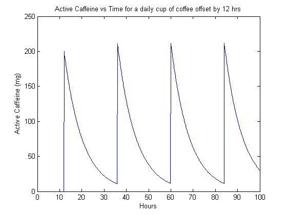
end

Let’s apply the code on some simple cases. The first thing we want to do is apply the model for a simple periodic dosing with some offset, just to confirm that the offset works correctly.

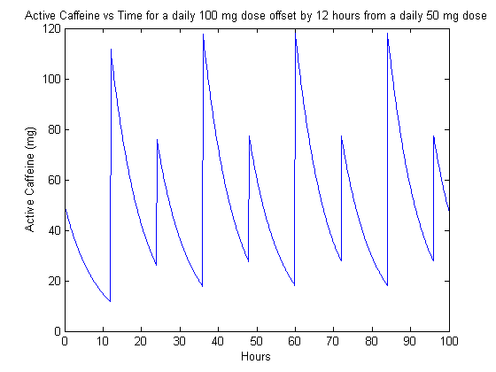
It appears like the code works. Now we look at a slightly more interesting case, a sum of two different dosing schedule. This example has a 50 mg dose at midnight ($t=0,24,48,\ldots$) and a 100 mg dose at noon ($t=12,36,60,\ldots$), where we have set $t=0$ as midnight.

Now we can try something more complicated and crazy looking. The next example has a periodic 50 mg dose every 12 hours, with an initial offset of 18 hours, a daily 100 mg dose with an offset of 9 hours, and another daily 100 mg dose with an offset of 14 hours. This complicated dosing schedule is handled easily by the MATLAB code, resulting in Figure 3.

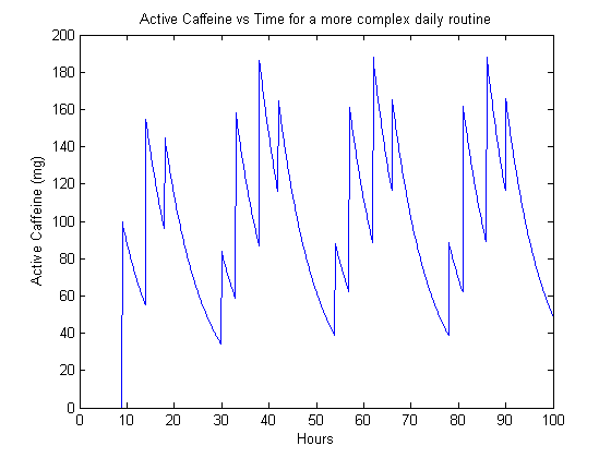
The infinite time behavior is now more complex, as the individual periodic functions may interfere with each other due to varying $a_j$ frequencies and $t_j$ offsets.

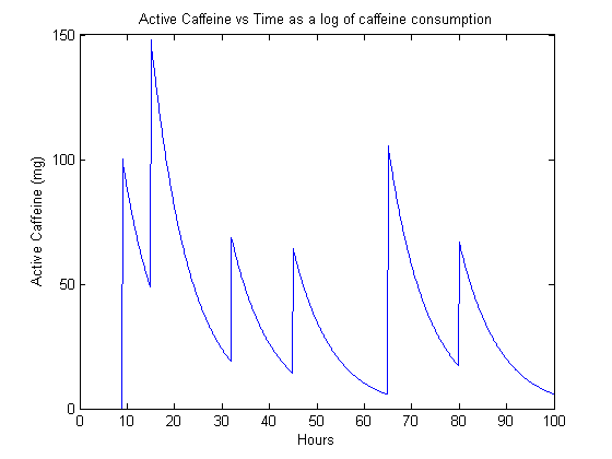
The next thing we look at is the special feature mentioned just before the code–the ability to include non-repeating dosages. This allows the program to act as a logbook of sorts to see what one’s caffeine levels might be. In this case, a list of inputs and offsets are provided where the offsets span the total duration of the time period of interest. In this case, we are no longer summing over many terms, so we can remove the summed geometric series from the expression and just replace it with the simpler exponential term.

As an example, the doses $[100,100,50,50,100,50]$ are associated with the offsets $[9,15,32,45,65,80]$, respectively. The resulting curve is plotted in Figure 4.

To summarize the results of this post: we expanded our method to handle arbitrary offsets and allowed for superposition of multiple periodic dosing regimens (and single doses) in order to be able to construct any possible dosing scheme. We looked at several different examples of periodic dosing schemes as well as completely manual logbook-style calculations.

Again, it must be stressed again that this is a toy model. Real systems don’t work this way, due to many physical effects and feedback systems within a person. It should also be noted that caffeine is used throughout as an example of interest, but it could be any other pharmaceutical drug that follows first-order exponential decay kinetics.