Modeling Caffeine Metabolism

Caffeine is a stimulant drug that is widely consumed in tea, coffee, soda, and chocolate, among other beverages and foods. In this post, we construct a toy model for caffeine metabolism.

The mechanism of action of caffeine is complex, as is the process of developing tolerance. These are important factors to consider when thinking about the ultimate effect of the drug on alertness and we will discuss them briefly at the end.

So–let’s build our model. We need to consider caffeine input (consumption) and caffeine output (metabolism).

For our caffeine input, let’s consider a semi-realistic model of consuming $d$ milligrams of caffeine as a single dose every $a$ hours. The simplifying assumptions associated with this model include the non-physical instant consumption of an entire source of caffeine under a rigid timeframe as well as neglecting the time needed for absorption within the body.

The instant consumption is not a terrible approximation since most sources are often consumed within 15 minutes or so. The rigid timefame is necessary to make the mathematics simple (as will be shown later), and is a more significant restriction. This model could not be used to consider someone who consumes a cup of coffee only at 9:00 am and 3:00pm every day, due to the periodic constraint on the caffeine input. This restriction imposes a constraint on the problems we can look at.

The assumption on the absorption of caffeine is a significant approximation. Typically, caffeine is absorbed through the intestine within 45 minutes of consumption with the peak blood caffeine content occuring between 1-2 hours after consumption. We have ignored these effects governing the bioavailability of caffeine. To justify this assumption, we can say that what our model is really looking at is the blood caffeine content with an instant input, i.e. instanteous absorption from the intestine into bioavailable forms that is time-shifted by some consistent amount after actual consumption. However, in a real system, there will be non-trivial dispersion of this input.

For our caffeine output (metabolism), we model the remaining active amount of the drug as an exponential decay with half-life 5.7 hours, based on the literature cited below. These assumptions are reasonable, given experimental data on caffeine content. Ignoring any prefactors, the significant tunable parameter for an exponential decay curve is the half-life (or equivalently, the time-constant). The half-life of caffeine in humans has been demonstrated to vary wildly depending on a variety of states of health. 5.7 hours is a reasonable mean value. The biochemistry underlying this decay is the degradation of caffeine into a number of other biomolecules, and follows first order kinetics.

We can now begin to put together our mathematical model.

First, the half-life of caffeine can be related to the time constant (for convenience) by

$\lambda = \tau \cdot \ln{2}$ $\tau=\frac{\lambda}{\ln{2}} = \frac{5.7}{\ln{2}}\textrm{hrs.} = 8.223 \textrm{ hrs.}$

This gives our simple exponential decay for a single dose of $d$ mg at time $t=0$ as $f(t)=d\cdot e^{-t/\tau}$ where $f(t)$ gives the amount of metabolically active caffeine.

We can now evaluate a sum of these terms that are each time-shifted by the time of intake of caffeine. As a simple example, for caffeine consumption at $t=0$ and $t=a$ , we have

$f(t) = d\cdot e^{-t/\tau} + d\cdot e^{-(t-a)/\tau}$

for all time $t\geq a$ since the second dose must be consumed for the equation to be valid.

For a more general sum at time $t=t_0$ , we need to sum the terms for all consumption events that have happened before $t_0$ . These events occur at time $t=0,a,2a,\ldots, n\cdot a$ where $na$ is the largest multiple of $a$ that is less than or equal to $t_0$ . We find that $n=\left\lfloor {\frac{t_0}{a}}\right\rfloor$ . Thus, we can write our sum as a sum of these decaying exponentials, with the number of exponential terms equal to the number of consumption events that have occured:

$f(t) = \sum_{i=0}^{n}{d\cdot e^{-(t-i\cdot a)/\tau}}$ $f(t) = d \sum_{i=0}^{n}{e^{-t/\tau} e^{i\cdot a/\tau}}$ $f(t) = d e^{-t/\tau} \sum_{i=0}^{n}{e^{i\cdot a/\tau}}$

We recognize the term within the summation to be a geometric series and replace the summation with the closed form sum.

$f(t) = d e^{-t/\tau} \left(\frac{1-e^{a(n+1)/\tau}}{1-e^{a/\tau}}\right)$

We now have our closed form expression for the active caffeine content. A direct observation that we can make is that the consumption dose acts as a scalar multiplier over the entire function.

What can we do with this expression? Well, we can use it to model several profiles of caffeine consumption. I implemented the model in MATLAB. The caffeine function takes in a single time point, the caffeine content of the source $d$ , and the duration between consumptions events $a$ and returns the active caffeine amount at that time.

function [ content ] = caffeine( time, caffeineContent, durationBetween )
    halfLife = 5.7;
    tau = halfLife/log(2);
    n = floor(time/durationBetween);
    content = caffeineContent * exp(-time/tau) * (1-exp(durationBetween * (n+1)/tau))/(1-exp(durationBetween/tau));
end

The caffeineList function takes in a list of times, $d$ , and $a$ , and returns a list containing the active caffeine amounts at the times indicated by the input.

function [ content ] = caffeineList( time, caffeineContent, durationBetween )
    content = zeros(1,length(time));
    for i = 1:length(time)
        content(i) = caffeine(time(i),caffeineContent,durationBetween);
    end    
end

The first thing we should do with this model is the trivial case of simulating a single dose. This acts as a sanity check to make sure that things look reasonable. This yields:

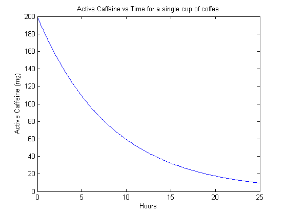
Figure 1: Response curve for a single cup of coffee equivalent at time 0.

Cool! It looks like the model works on this trivial case. Now we can look at more interesting cases. The next example is a coffee-cup-equivalent every 24 hours.

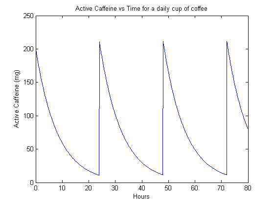
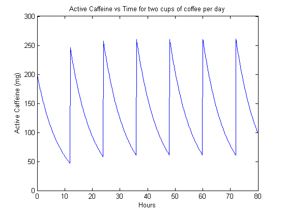
Figure 2: Response curve for a daily cup of coffee equivalent.

We can now look at someone who drinks coffee twice a day. Unfortunately, we’re forced by our formalism to stick to doses that are 12 hours apart, which is perhaps not the most realistic model for how people consume coffee, but still perhaps worthwhile to look at.

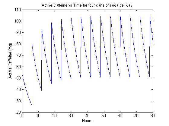
Figure 3: Response curve for two cups of coffee equivalent per day.

Now, we look at frequent consumption of a smaller dose of caffeine. Our model here is four servings of 54 mg of caffeine, simulating the extreme consumption of four cans of soda per day.

Figure 4: Reponse curve for four cans of soda equivalent per day.

Now we can think about the results a bit. First, the shape of the curves is entirely unsurprising–this is what a train of exponentials looks like. The result may be familiar from circuit theory.

We have two time-scales to look at: the steady-state and the transient.

The steady-state is perhaps more interesting, simulating the behavior of a habitutated drinker. We can see that in the case of 1 cup of coffee per day (figure 2), the caffeine content actually dips quite low before the next dose. However, when the drinker goes up to two cups per day (figure 3), they have a significant background level of active caffeine that is around 60 mg. This means that that much caffeine is constantly active in their bodies.

In the case of the transients, we can think of this as someone coming back to caffeine consumption after a long period without any consumption. The transition from no consumption to steady-state is perhaps clearest in figure 4. Here, we see the rise in background up to about 50 mg of always active caffeine (nearly a can of soda equivalent).

Remember, this is a toy model and shouldn’t be used for quantitative predictions. Qualitatively, we can clearly see that frequent consumption leads to a significant background level.

We can briefly consider the biological side of things. The mechanism of action of caffeine is to act as a competitive inhibitor on certain receptors within certain neurons. An increased background level of cafffeine means that the caffeine is constantly acting on these receptors as a competitive inhibitor. In a realistic biological system, this activity may change the profile of gene expression to increase receptor production, requiring more caffeine to result in the same effect, i.e. tolerance to a certain dosage of caffeine.

It is important to note that the relationship between our computed curves and complex physiological effects such as increased alertness is very complex. From our model, we really cannot say much with any certainty about this relationship, due to the complexity of the relationships between amounts of the drug, its biochemical activity, and its effect on behavior. There may be complex feedback regulation at multiple levels that makes this relationship complex and beyond the scope of this simple model.

To summarize: we have built a toy model for caffeine metabolism and used it to evaluate several different profiles of caffeine consumption, with a perspective towards the underlying biochemistry.

Disclaimer: this is not medical advice. The information in this post is not intended to diagnose, treat, cure, or prevent any disease.

References

“Serum caffeine half-lives. Healthy subjects vs. patients having alcoholic hepatic disease.” Am J Clin Pathol. 1980 Mar;73(3):390-3. PubMed
“Plasma and salivary pharmacokinetics of caffeine in man.” Eur J Clin Pharmacol. 1981;21(1):45-52. PubMed
Wikipedia page on Caffeine.

Written on December 30, 2014